
We examine a potential solution to the funding dilemma that defined benefit pension plans face – the Variable Annuity Pension Plan (VAPP). Our analysis highlights the need for greater insight regarding asset-liability matching, and points out that transitioning to a VAPP can benefit from new and critical thinking on the management of plan assets.
Investments and the Evolution of Defined Benefit Pensions
Stories abound telling us how poorly prepared financially many Americans are for retirement. Apart from Social Security, most workers will not receive a guaranteed benefit payment on retirement. Much of the problem of being financially unprepared can be attributed to the demise of traditional pension plans.
There are two general forms that a pension can take: traditional defined benefit (DB) plans, which promise a set stream of payments to a retiree for the remainder of his or her post-retirement life; and defined contribution plans (DC), which allow participants to accumulate assets for their own individual retirements. Over the last few decades, DC plans have largely supplanted DB plans, except for public sector workers (e.g. state and local employees) and unionized private sector workers. According to the Bureau of Labor Statistics (BLS), in 2018 only 12% of non-union private sector workers was covered by a traditional defined benefit pension plan, compared to 68% of union workers in the private sector. Although DC retirement plans are increasingly popular, DB pension plans have several advantages over the DC plans. A DB plan benefits by spreading longevity risk (i.e. the risk of outliving your assets) across all participants, so no individual participant is in danger of “running out of money”. How much a person needs to have saved by retirement is a function of: their life expectancy, their income needs, and the likely returns that their portfolio will generate.
“In 2018 less than one in eight non-union private sector workers was covered by a traditional defined benefit pension plan.”
The average life expectancy of a large group of people is more easily predicted than is the life expectancy for any given individual. As a result, a DB pension can more accurately estimate the amount of money needed to fund retirement income for a large group of participants than an individual can estimate the amount they need to save in their DC plan.
Income and spending in retirement is also an area in which DB plans provide an advantage over DC plans. Because the DB income payments (typically monthly) are stable and predictable, retirees can easily understand how much they can safely spend. With a DC plan, most retirees will have no idea what the “supportable” withdrawal rate is; in other words, how much money they can safely take from their portfolio each month.
Forming expectations about the last variable, portfolio returns, is arguably the most difficult, and is probably the most overlooked. Producing a realistic expected return requires formulating an asset allocation and reasonable return estimates for each asset class. In addition, the expected return needs to be adjusted for any difference between the asset class return forecasts and the actual returns earned by the portfolio after taking into account fees and implementation costs.
Current Issues with DB Plans
The state of the remaining DB plans illuminates some of the issues that have driven companies to adopt DC plans, despite the advantages of DB plans to employees. Over the last two decades, and especially since the global financial crisis, many DB plans have become underfunded, meaning that the assets in the plan are projected to be insufficient to cover the promised benefits.
In the case of public employee pensions, the cause of the funding trouble has often been a failure of governments to make the necessary contributions to the plans. In extreme cases, funds have been impacted by sponsor insolvency. When the entity responsible for contributing to the pension can no longer make those payments, the odds increase that the promised benefits cannot be paid. Examples include: United Airlines (corporate, 2005 bankruptcy) and Detroit (public/municipal, 2014 bankruptcy). For the Central States Teamsters, a multi-employer pension, much of the deficiency can be traced to the massive number of trucking bankruptcies after early 1980s deregulation.
One of the primary drivers of the shift away from DB plans has been investment risk. All plans face the risk that the returns on plan assets fall below expectations. In a traditional DB plan, the sponsor bears the risk that the investment portfolio fails to generate returns sufficient to pay the promised benefits. Many plans have relatively high return assumptions, increasing the likelihood that asset pools will be unable to deliver those results in today’s financial market environment. In particular, prospective returns in bonds are very low, given the current historically low level of bond yields.
The trouble for a number of other multi-employer plans has been lower than expected returns on plan assets when the tech bubble burst in the early 2000s and equity markets fell during the global financial crisis in the late 2000s. These poor returns came after the late 1990s, when benefits were often increased in order to alleviate an overfunded situation, which could have jeopardized the tax-deductibility of employer contributions. Due to the negative equity returns during these periods, the realized long-term returns for many plans (despite their bond holdings and diversification) have turned out to be below expectations and insufficient to meet their benefit obligations.
In an attempt to generate higher returns in the wake of the financial crisis, many funds introduced new allocations, or increased existing allocations, to esoteric alternative assets. Unfortunately, this was not the panacea that was hoped for, as the performance of many of these investments fell short of expectations.
Structure of the Traditional DB
A traditional DB has “fixed” benefits; in other words, stable monthly benefit payments during retirement until death. In order to pay these promised benefits, a sponsor must contribute sufficient assets to the plan, generally as the benefits are earned.
If a plan does not set aside sufficient assets or fails to achieve its required rate of return, it will become underfunded and therefore must either cut benefits or increase contributions (or some combination of the two).
There are a number of different ways that an underfunding problem can arise. One is that the amount of benefits can be underestimated. Actuarial assumptions about longevity of participants 30 or 40 years in the future are inherently uncertain, and any underestimate of lifespans can lead to an underestimate of the necessary contribution level. Another problem is overestimating the rate of return on plan assets. Many plans will formulate a forward-looking return assumption on the basis of what returns looked like in the past. This can produce an overly optimistic view of how much the asset portfolio will appreciate each year. Consider the secular decline in bond yields during the 1980s and 1990s. Yields on long-term Treasury bonds began this period around 15% and fell for the next two decades. As a result, bond returns were very high, benefitting from a combination of generous coupon income plus the capital gains generated as bond yields fell and prices rose. Incorporating this time period into the estimate of future bond returns would result in overly optimistic expectations given today’s relatively low yields.
Compounding the asset return problem is the fact that plans can see their actual portfolio performance fall short of what the financial markets provide. One of the drivers of this underperformance can be cash flows. When financial markets fall, but benefit payments to retirees are fixed, the outflows as a percentage of fund assets get larger. This means that the poor portfolio performance gets amplified in its effect on the fund’s market value. Unfortunately, the problem of cash flows affecting returns is unavoidable.
A plan’s ultimate concern is the monetary return generated on the assets in its portfolio. When the fund experiences cash flows and returns are volatile, the dollars generated will not necessarily be the same as the percentage return multiplied by the market value of the portfolio. Consider the two mature pension plans shown in Table 1. Both start the 10-year period with $100 million in assets, and both experience total cash outflows of $45 million over the 10 years (i.e., average annual net benefit payments of $4.5 million). Plan 1 enjoys a consistent return of 6.5% each year for the 10 years. Plan 2 experiences an identical time-weighted (geometric average) return of 6.5%; unfortunately, this is composed of a mix of good and bad years. The net benefit payments are uneven, with bigger outflows for Plan 2 occurring in years of poor financial markets and smaller outflows during good years. The ultimate outcomes for the two plans are quite different: Plan 2 ends up with assets nearly $19.5 million below the assets of Plan 1, and therefore with a much weaker funding status.
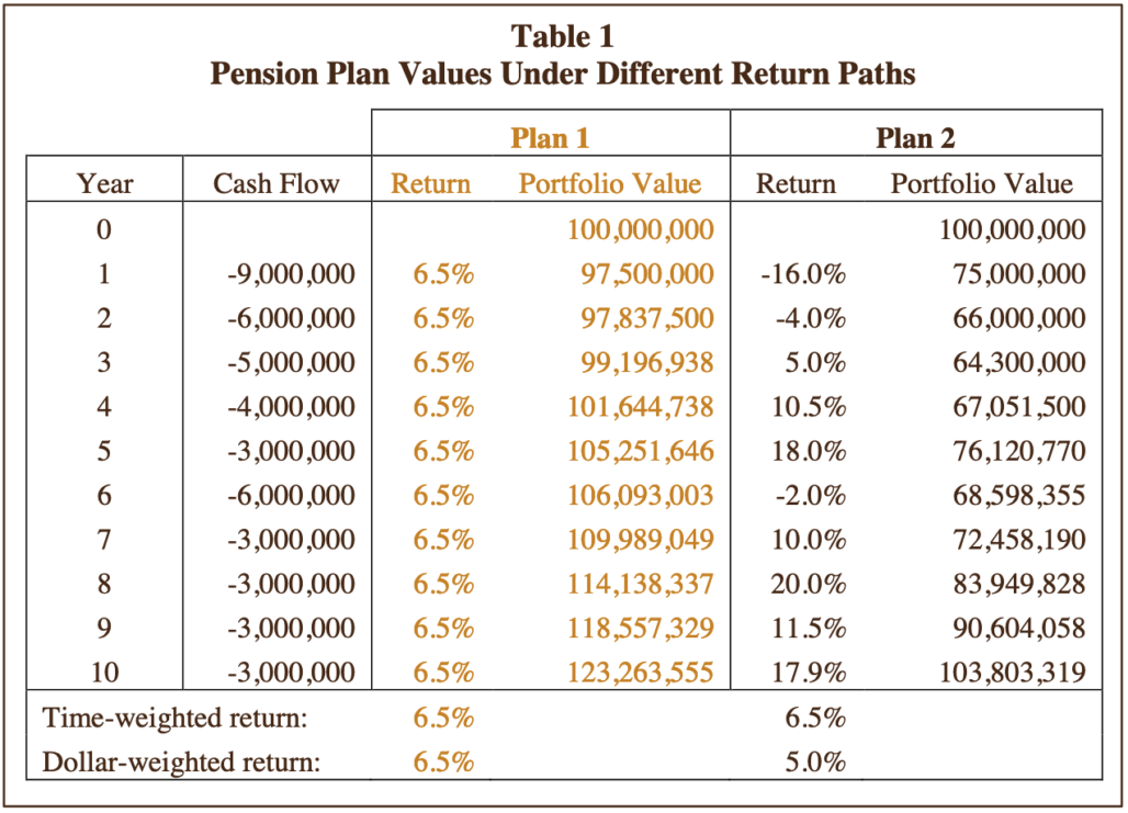
In effect, as the risk increases in a portfolio that is subject to cash flows, there is a corresponding increase in the difference between the returns measured on a periodic basis (i.e. time-weighted) and the returns measured in dollar terms (dollar-weighted or IRR). While time-weighted returns are generally appropriate for evaluating investment performance, dollar-weighted returns have a direct impact on plan assets and therefore the funding status of the plan. We estimate that over time the gap between financial market returns and actual fund experience can be a full percentage point or more per year. In other words, a fund that would have grown its assets by its return of 6.5% if the assets had been left “untouched,” will in practice generate a lower return in dollar terms when withdrawals are made in poor market environments. In the example above, although the annualized time-weighted return for both plans is 6.5%, the dollar-weighted return of Plan 2 is 1.50% below the dollar-weighted return of Plan 1.
“We estimate that over time the gap between financial market returns and actual fund experience can be a full percentage point or more per year.”
This difference between time-weighted and dollar-weighted returns is larger when the portfolio’s returns are more volatile and when negative cash flows occur at times of losses when the portfolio’s value has declined. Given their cash outflows, mature plans will be more susceptible to funding problems arising from poor financial market performance than young plans would be. This has real-world implications, as evidenced by the Department of the Treasury’s rejection of the Central States Teamsters Plan’s application to reduce benefits. In its letter to the Teamsters Plan1, Treasury denied the proposal, in part because the modifications were unlikely to meet the requirement “that the proposed benefit suspensions be reasonably estimated to allow the plan to avoid insolvency.”2 Even with benefit reductions, the plan would not be solvent when faced with a combination of poor returns and large net outflows.
Specifically, Treasury deemed the plan’s return expectation of 7.5% to be overly optimistic, particularly in the near term when considering relevant current economic data. In addition, the plan had not taken into account: “the timing of future expected contributions and benefit payments, which…results in the Plan having significant negative cash flow and therefore declining asset levels. …these projections are extremely sensitive to variations in asset returns in the near term because the same percentage gain or loss has a greater impact if it occurs earlier, when asset levels are higher, than in later years, when asset levels are lower.”3
Compounding the cash flow problem, some plans try to make up for past underperformance by increasing their portfolio’s future returns rather than by increasing contributions. In most cases, this approach will not solve the underfunding problem. Clearly, one of the biggest issues with this approach to closing the funding gap is that increased risk could result in even more severe underfunding if markets decline. Generating higher returns is unlikely to suffice for closing a funding gap, unless that gap is very small. Consider a plan that is 70% funded: if the return assumption is 7.5% annually, the return that would be needed just to keep the funding status stable is 10.7% every year! In simple terms, this is because only 70% of the assets are available to generate returns, meaning the portfolio would have to deliver a much higher return in order to provide the same benefit. Ultimately, if there is a substantial shortfall in a DB plan’s ability to pay promised benefits, then contributions will likely need to be increased. For multi-employer plans, this results in current active participants subsidizing retirees and older workers whose benefits were accrued under the overly optimistic assumptions.
Other Considerations
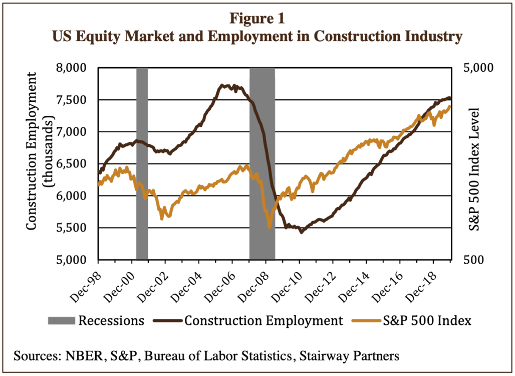
It is worth noting that contribution levels are often tied to the health of the economy, which can exacerbate a funding problem. In an economic recession, employment in construction and manufacturing typically declines sharply, which reduces pension fund contributions for plans that are funded based on hours worked. In addition, workers who are older but still active might retire, effectively increasing the fund’s benefit payments.
Unfortunately, as Figure 1 shows, a weak economy and falling employment are typically also accompanied by a falling equity market, which exacerbates pension funding and cash flow problems.
As mentioned, one way some DB pension sponsors have tried in the past to address their return shortfall has been to increase the risk and expected return of the portfolio. Although this increases the long-run expected return, it can also mean an increase in the likelihood of running out of money due to the greater riskiness of the portfolio, especially in the face of reduced cash flows.
Simulations
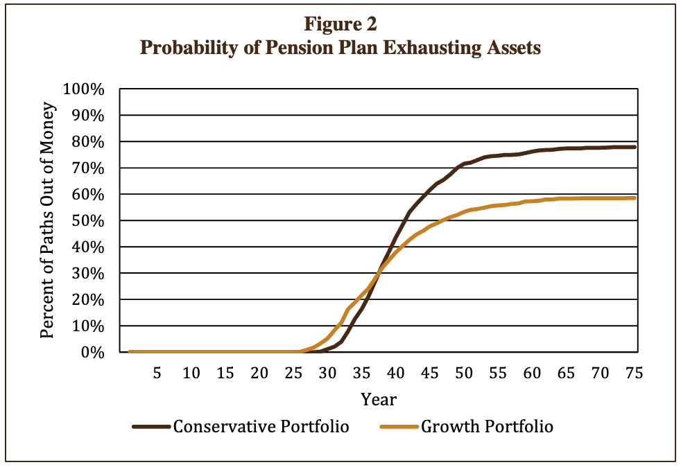
We used Monte Carlo simulation to analyze a DB plan’s financial characteristics under volatile financial markets. Monte Carlo simulation is a technique for creating a series of portfolio returns, based on random sampling from the return distributions of the portfolio’s asset classes. This allows us to generate a large number of portfolio returns that have characteristics consistent with the component asset classes’ returns, risks, and correlations. One advantage of the Monte Carlo technique is that it is not tied to historical data that are limited in scope and are not always representative of expectations of future returns. Another benefit of using Monte Carlo is that it allows us to examine the effects of cash flows on the range of portfolio outcomes. For this analysis, we generated 1,000 return paths for two portfolios: a fully funded Conservative portfolio with a long-run expected annual return of 6.8% and risk (annualized return volatility) of 7.9%, and a Growth portfolio with an expected return of 8.0% and risk of 14.1%.
Figure 2 shows the percentage of times that the two portfolios exhaust their assets before all benefits are paid. Higher risk and expected return results in fewer paths running out of money in the long run (i.e. lower percentage of paths, due to the higher average return) but a higher percentage running out of money over shorter time periods (due to the short-run effect of higher risk on the portfolio’s value).
Variable Annuity Pension Plans
Rather than increasing the plan’s risk in an attempt to meet lofty fixed return assumptions, some multiemployer plan sponsors are taking steps to implement Variable Annuity Pension Plans (VAPP). With a VAPP, benefit levels are tied to the performance of the assets, so that the risk and return of the portfolio feeds directly through to the participants’ benefits. Typically, the assumed long-term return used to set the VAPP benefit accrual will be more conservative than the traditional DB return assumption, for instance 4.5% rather than 7.0%. However, if the asset portfolio generates long-term returns higher than the reduced return hurdle, the benefit will be adjusted upwards over time. Conversely, if poor financial market performance results in the portfolio experiencing returns less than the hurdle, participants could see their benefits cut below the already-lower accrual rate. Although returns can be volatile and result in portfolio losses during some periods, the lower VAPP return hurdle greatly reduces the likelihood that the assets are insufficient to pay the low accrual-rate benefits. The likelihood of running out of money is essentially eliminated when benefits can actually be reduced below the accrual level benefit.
Given the sensitivity of benefit accruals to short-term investment returns, we believe that investment portfolio design should be a critical component of VAPP design.
The plan trustees’ primary decision is to determine the overall level of risk and assumed return for the portfolio. The asset decision hinges on the tolerance for benefit variability weighed against the desire for long-term growth in benefits.
Like a DC plan, a VAPP essentially shifts much of the investment risk from the plan sponsors and active participants to all participants, including retirees. However, the VAPP maintains several of the key advantages of DB plans:
- The participants are not individually exposed to longevity risk because it is spread across a large pool of participants.
- The risk of employers pulling out of a fund (withdrawal risk) is greatly reduced because a VAPP is designed to be fully funded at all times.
- The plan participants benefit from professional management.
A significant challenge for those seeking to implement a VAPP is the need for participants to understand and accept the possible variability of their future benefits. Hopefully, the many news stories about public and multi-employer plans facing dire funding situations will help participants see the desirability of ensuring that their retirement plan does not end up in a similar situation.
VAPP Features and Tradeoffs
When designing a VAPP, it is possible to incorporate one or more mechanisms to mitigate the likelihood that benefit levels get reduced below the low base accrual rate. These mechanisms can include: return smoothing or creating a reserve pool. Each of these mechanisms has pros and cons
Return smoothing involves adjusting benefits by an average of previous years’ returns rather than a single year. A smoothed return will almost certainly limit the frequency and magnitude of benefit reductions relative to the simple full-adjustment VAPP. However, one of this mechanism’s potential weaknesses is the possibility that the plan becomes underfunded.
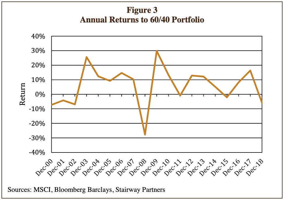
As an example, we analyzed the returns of a 60% equity/40% bond portfolio. This portfolio’s 5-year average return at year-end 2006 was 10.5% and year-end 2007 was 14.3%. With five-year smoothing, this would indicate that benefit payment amounts would have been boosted by almost 16% in the span of only two years (the excess of the returns above a 4.5% hurdle rate).
For the sake of argument, assume that the plan’s demographics were heavily skewed toward retirees (a small proportion of active participants). If that were the case, the benefit payment outflows from the plan would have increased considerably just as equity markets globally were hitting a rough patch. In 2008, the benefit accruals would be based on the 14.3% five-year average return through 2007. However, as shown in Figure 3, the actual return to the portfolio in 2008 was -27.8% due to poor equity market returns. The poor performance of the assets, when coupled with the larger outflows from the enhanced benefits, could have endangered the plan’s funding status.
This example also points out another potential drawback of any type of smoothing mechanism: when smoothing exists and the plan is experiencing cash flows (either significant contributions or benefit payments), some group of participants can end up subsidizing another group. For instance, if the benefits calculated using smoothing are below the benefits calculated using a pure VAPP framework, the plan will be overfunded and retirees will be “subsidizing” active participants. Conversely, as in the late 2000s example above, if the benefits with return smoothing exceed the pure-VAPP benefits, then the payments to current retirees are “excessive” and drawing down the plan. As the plan becomes less than fully funded, the retirees are being subsidized by active participants. Ultimately, return smoothing can reintroduce some of the DB funding issues that the pure VAPP was designed to avoid.
Reserve pool is a feature that includes funding a reserve balance that is used to “top up” benefits when poor asset returns would have otherwise caused them to decline. The reserves can be pre-funded at the start of the VAPP program or reserves can be funded through regular contributions as benefits are accrued. In addition, the reserve can be funded by “capping” benefit increases during periods of strong market performance, with the excess return over the cap going to the reserve pool. For example, the cap might be set at 10%, so that the annual benefit increase is limited and the “excess” return on the portfolio is moved to the reserves. When the portfolio’s return falls below the base return hurdle (e.g., 4.5%), reserves are moved back to the portfolio in order to shore up the benefit. As is the case with other mechanisms, having a reserve cannot ensure with 100% certainty that benefits will not decrease. Consider again the financial market environment during the crisis a decade ago. A pool of reserves that was as large as 30% of the main portfolio could have been fully drawn down. In 2008, when the 60/40 portfolio lost nearly one-third of its value, this could have necessitated reducing benefits until financial markets rebounded sufficiently to allow benefit levels to be adjusted back up.
Segregating reserves can allow a plan sponsor to use a more targeted approach to risk management. For example, having a pool of reserves managed in a low-risk fashion allows the main VAPP portfolio to take a somewhat more aggressive stance in its investment program. The reason for managing the reserves conservatively is straightforward: if reserves are intended to act as a buffer for times when financial markets are doing poorly, then the reserves should not be losing value when they are most needed.
We also used Monte Carlo simulation to investigate how adding a reserve pool to a basic VAPP might mitigate some of its drawbacks, particularly the cuts to benefit levels when financial markets perform poorly. For the VAPP simulation, we generated 1,000 return paths for a moderate-risk portfolio, like the 60/40 portfolio in the prior discussion, over 60 years (35 years of working/contributions and 25 years of retirement/benefit payments).
Using our setup, we looked at several important variables, including the size of the reserve pool and the riskiness of the portfolio. The analysis shows that increasing the potential size of the reserve provides for a smoother benefit path. If reserves can be tapped to top up the main fund any time it declines in value due to a poor return, benefit levels and accruals do not need to be cut. And when returns are very strong above a return cap the excess is transferred to the reserve. Because we assume a low cash-like return for the reserve pool, the “cost” of holding reserves shows up as a lower return overall for the combined main pool and reserve pool. This can be offset to some extent by increasing the risk and expected return of the main pool. However, this does modestly increase the likelihood of very poor returns exhausting the reserve pool.
Figure 4 shows the benefit of having a reserve. Under the basic VAPP, benefit accruals vary directly with the performance of the asset portfolio. As a result, there are periods of substantial declines in value of both the portfolio and therefore the accrued benefits. A drawdown is the cumulative decline in a portfolio’s value from peak to trough. In Figure 4, the brown-shaded columns show the largest drawdown experienced by the basic VAPP in the simulation paths. More than half of the paths had a drawdown of greater than 22%, and one out of four paths experienced a drawdown of more than 30% at some point during the 60 years. We imagine that participants would be shocked to see their benefits (promised or actual) fall by that much.
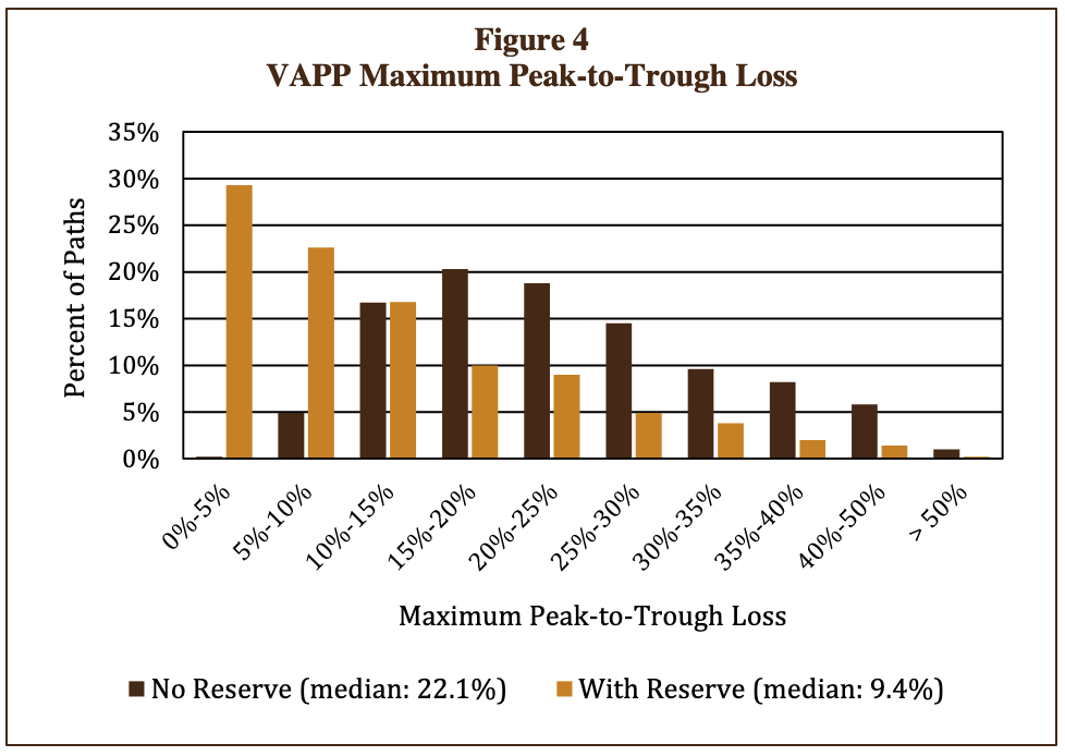
When a reserve pool is put in place, the likelihood of a reduction in benefit accruals is greatly reduced. (In this case, the reserve pool was allowed to grow to 35% and the return cap was set at 10%.) With the reserve feature in place, half of the paths show the portfolio losing less than 9.4% at its worst point, compared to losses of more than 22% without the reserve. Over two-thirds of the paths have a maximum drawdown of less than 15%. Although holding reserves to stabilize the benefit accruals has a clear advantage in limiting benefit cuts, there is an explicit cost. We estimate that investing the reserves in minimal-risk, and thus low-return, assets (such as cash and very short-duration high-quality bonds) reduces the ultimate benefit accrual growth rate by 50 to 100 basis points (one-half to a full percentage point), compared to a fully variable VAPP.
A plan’s sponsor is ultimately responsible for choosing a point on the continuum between avoiding cuts to benefit accruals and having them grow strongly over time. The important variables include the base accrual rate, the size of the reserve, the risk and return of the main asset portfolio, and the return cap. Each of these factors will influence the average rate of accrual and the related likelihood that benefits and accruals are reduced.
When evaluating a VAPP, the sponsor should also consider the types of assets to be included in the main portfolio. Because benefits are tied directly to the performance of the assets, good returns will eventually result in benefit improvements and poor returns will result in benefit cuts. However, consider what could happen if the portfolio includes an allocation to illiquid investments, where pricing is uncertain. Because these investments are valued based on appraisals or estimates, their returns might not reflect their true underlying economic value. For example, during times of financial market distress when publicly traded asset prices are falling sharply, assets in an untraded illiquid structure might not get marked down in a timely manner. If the prices of these illiquid investments are overstated, the returns and participants’ benefits will also be overstated. Retirees will benefit and active participants will be disadvantaged, as fund resources are shifted from those contributing to those who are receiving benefits. When this occurs, there is an inadvertent transfer of wealth from one class of participants to another. Because illiquid investments tend to smooth the overall portfolio’s returns, the result is similar to the wealth transfers that arise when returns are explicitly smoothed in determining benefit levels.
Conclusion
Our analysis highlights the need for better insight and understanding regarding asset-liability matching, and points out that transitioning to a VAPP can benefit from new thinking on the management of a plan’s assets. By raising these issues, we hope to help pension plans considering the adoption of VAPPs avoid some of the pitfalls that have created problems in the past.
Ultimately, we believe that the manner in which the investment portfolio is managed should be a function of the VAPP’s design. With a smoothed benefit design, it might make sense to take a lower-risk approach in managing the asset portfolio. This would mitigate some of the underfunding risk and the potential for inadvertent transfers between retirees and actives. The plan trustees would need to recognize that this comes at a cost of reduced growth in expected benefit levels.
With a reserve pool feature, it likely makes sense to manage the main portfolio with a higher-risk/higher-return objective, in order to capture the higher expected growth in benefit levels over time. In contrast, the reserve pool is probably better targeted toward a low-risk policy one that ensures the reserves do not decline in value when they are most needed.
Finally, regardless of the actuarial approach chosen, when designing an investment portfolio for a VAPP, the plan sponsor should understand the impact that variable cash flows and return volatility could have on plan assets.
Footnotes
- Letter dated May 6, 2016 to Board of Trustees, Central States, Southeast and Southwest Area Pension Plan from Kenneth R. Feinberg, Special Master, Department of the treasury(“CST Letter”)
- CST Letter, page 1
- CST Letter, page 4
Stairway Partners, LLC © 2020
This material is based upon information that we believe to be reliable, but no representation is being made that it is accurate or complete, and it should not be relied upon as such. This material is based upon our assumptions, opinions and estimates as of the date the material was prepared. Changes to assumptions, opinions and estimates are subject to change without notice. Past performance is not indicative of future results, and no representation is being made that any returns indicated will be achieved. This material has been prepared for information purposes and does not constitute investment advice. This material does not take into account particular investment objectives or financial situations. Strategies and financial instruments described in this material may not be suitable for all investors. Readers should not act upon the information without seeking professional advice. This material is not a recommendation or an offer or solicitation for the purchase or sale of any security or other financial instrument.

You must be logged in to post a comment.