A well-constructed portfolio should, over time, provide investors with a good chance of achieving their investment objectives.
Hitting a Target Return: Swing for the Fences?
Whether they recognize it explicitly or not, all investors put money into portfolios to cover future liabilities or spending goals. Pension funds provide workers with retirement benefits. Insurance companies hold money to pay claims. Individuals save money to provide for things like retirement and their children’s education expenses.
Ideally, an investor with liabilities wants their portfolio to provide a rate of return sufficient to meet the liability when it comes due. This rate of return is known as a hurdle rate or required return. The best asset would be one with a return that matches or exceeds the required return, but has no risk that it would underperform the hurdle.
Unfortunately, the perfect asset – one that meets the required return with no risk – rarely exists in the real world. Investors will typically need to take risk in order to generate an expected return high enough to meet their required return.
Liabilities
Many investors have liabilities that grow at a rate that exceeds the general inflation rate as measured by the Consumer Price Index (CPI). For example, a traditional single-employer defined-benefit pension might guarantee payments in retirement that are a function of an employee’s final five years of earnings. Salaries tend to rise faster than inflation, as an employee’s seniority and productivity increase over time. Likewise, for many years the cost of college has risen at a much faster rate than CPI inflation, which has increased the difficulty of saving enough money to pay for a child’s college education. Over the last 20 years, the overall CPI inflation rate has averaged 2.2% per year. In contrast, the CPI series for tuition has increased at an average annual rate of 5.2%. This means that if $1,000 had grown in line with the general CPI for the last twenty years, it would amount to a bit above $1,500 now. In contrast, the amount of tuition that $1,000 bought twenty years ago would now cost well in excess of $2,700, an increase that is more than triple the increase of prices overall.
To make matters worse, the liabilities are often uncertain: no one knows exactly how much their 10-year-old child’s college tuition will cost in 8 or 10 years; and, in planning for retirement, no one knows what their life span will be. There are averages and educated guesses, but no certainty when it comes to liabilities.
Investment Alternatives
If an investor could afford to purchase a sufficient quantity, a default-free government bond that matures at the same time as the liability comes due would be the ideal investment. When an investor is able to assemble a portfolio that contains enough bonds to pay off the liabilities at the appropriate time, we say that the portfolio “immunizes” the liability. There is no risk that the investor will not have enough money to satisfy the liability.
With the 10-year government bond yield around 2.50%, few investors have a large enough portfolio to purchase a sufficient amount of bonds to cover their liabilities. Put another way, their required return is above the very low yield on default-free government bonds. If the portfolio is insufficient to immunize the liabilities, the investor will either need to contribute additional money or they will need to take risk in the portfolio to try to boost returns above the yield on government bonds.
“Riskier/higher return portfolios are appropriate for investors with longer time horizons, despite the greater likelihood of poor returns over shorter time periods”
In practice, the vast majority of investors will be unable to contribute sufficient additional money, so they will need to hold “risky” assets in their portfolios. These assets have higher expected returns over time. But, they also have returns that fluctuate – sometimes over a wide range – around the long-term expected return. Because the future is uncertain, there will always be a risk that, even over the long run, a portfolio’s return may fall short of the hurdle return.
One-Year Horizon
To illustrate this point, we will start with a one-year horizon. Assume that you have $38,000 set aside to pay a $40,000 education expense in one year. If there will be no further contributions to the pool of money, you will need this portfolio to grow by 5.25% in order to pay the tuition in one year.
Unfortunately, the 1-year Treasury bill currently provides a return of only 1.5%. So, if you are not willing to be exposed to any risk, you will end up one year from now more than $1,400 (or about 3.75%) short of money. (This is the difference between what is required to fund the liability and what will actually be earned on the investment.) In order to have a chance of achieving the 5.25% target, you will need to hold assets that have returns above risk-free Treasuries, for example, by allocating some of the money to equities instead of Treasuries. The other alternative is to add another 3.75% to the portfolio so that you would have sufficient money to fund the education expense a year from now.
Assume that the long-term expected return on equities is 8.0%. We would need to hold a moderate-risk portfolio of around 60% equities and only 40% Treasuries in order to achieve the 5.25% return. But, because equity returns fluctuate over shorter periods, there will be a real possibility of falling short of the 5.25% target. Rather than a 1.5% return with certainty, there is uncertainty associated with the higher expected return on equities. Note, however, that if you were to hold only risk-free Treasuries, the probability of falling short is 100%!
Although the “average” expected return on equities might be 8.0%, there is a wide range of possible outcomes around that number. In technical terms, the average is the center of a wide distribution. For simplicity, assume that equities have a standard deviation of returns of 15% over one year. This means that 68% of annual equity returns are expected to fall within a range of -7.0% to +23.0% (8.0% ± 15.0%). This range might seem fairly wide, but it also means that about one-third of the time the equity return will be lower than -7.0% or higher than 23.0%.
When we combine equities with the risk-free Treasury investment, the 5.25% expected return is a weighted average of the two returns. Likewise, the portfolio that blends the two assets will have a standard deviation that lies between the two standard deviations. In our example, the standard deviation of returns of the blended portfolio would be 9.0%. In other words, two-thirds of the time we would expect the portfolio’s returns to fall in the range 3.75% to +14.25% (which is the 5.25% weighted-average return ± 9.0% standard deviation). Stated a different way, because the expected return is approximately equal to the target return, half of the distribution lies above the 5.25% target and half below. So in any given year, we would expect about a 50-50 chance of meeting or exceeding the target. In Figure 1, we depict the portfolio’s expected return graphically.
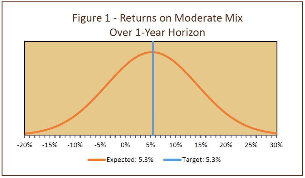
To improve the likelihood of meeting or exceeding the target, the portfolio’s expected return needs to be above the target return. That means (in this simple example) adding more higher-returning equities to the mix, with a commensurate reduction in low-return Treasuries. Unfortunately, this also means that the riskiness (the variability of possible outcomes) of the portfolio will increase.
If we boost the equity portion from 60% to 90%, the expected return will rise from 5.25% to 7.35%, providing a decent margin over the target. However, the portfolio’s risk also increases substantially, from a moderate level to an aggressive level. This means that we should expect a much greater fluctuation of returns around the new 7.35% average return; the standard deviation will increase from 9% to 13.5%. So our two-thirds range of returns widens from -3.75%/+14.25% to 6.25%/+20.85%. Although larger positive returns have become more likely, so have larger negative returns. This is shown in Figure 2 by the “higher” level of the curve at large positive and large negative returns (compared to the returns in Figure 1).
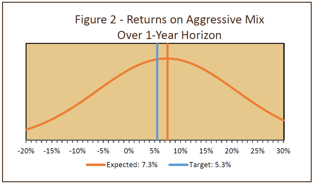
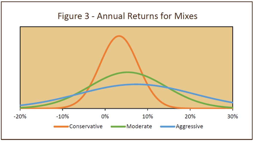
Figure 3 shows that, as the equity portion of the portfolio is increased – from 30% for a conservative portfolio, to 60% for a moderate-risk portfolio, and to 90% for an aggressive portfolio – the expected return increases (the peak of the curve shifts to the right). However, large returns – both gains and losses – become more likely.
Given the increased range of returns around the average return of 7.3% on the aggressive portfolio, what has happened to the likelihood of achieving the 5.25% target? It seems reasonable to think that the probability is higher than 50%, because the center of the distribution is above the target. In fact, this is what happens. Mathematically, the likelihood would be about 56% that the 90/10 mix has a return in excess of 5.25%.
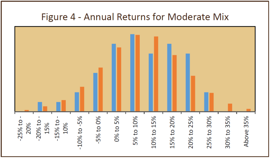
How does the historical record look compared to this hypothetical setup? Figure 4 shows a histogram of the pattern of annual returns that we would expect from our aggressive mix (in orange), compared with that of actual annual returns from 1973 to 2016 (in blue). Actual returns have not followed a smooth normal distribution, although they are roughly similar to our hypothetical distribution.
Longer Horizons
What happens if we extend the time horizon beyond one year? Over time, markets tend to revert toward a fairly priced level. So if returns are very strong for an extended period and prices get unsustainably high, subsequent returns are likely to be poor. The reverse is also true. When investors are overly pessimistic, creating an environment of cheap asset prices, subsequent returns will tend to be strongly positive as prices recover.
This means that, over longer periods of time, extreme returns (either positive or negative) tend to get dampened down, resulting in somewhat lower long-term volatility. Given the lower dispersion of (annualized) returns, the probability of achieving the target return is altered. Recall that using our example of an aggressive 90:10 mix of equities and Treasuries, there was a 56% chance of exceeding the 5.25% target in a single year. Because the mix has an expected return that is above 5.25%, if we extend the time horizon to 5 years, the probability of exceeding the target rises from 56% to nearly 69%.
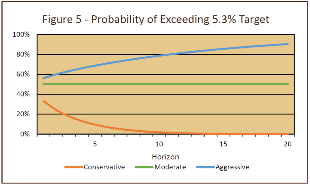
As Figure 5 shows, the likelihood of the return on the aggressive portfolio exceeding the 5.25% target increases as the time horizon is lengthened. Although the probability is only 56% for a one-year horizon, those better-than-even odds cumulate over time. In contrast, the conservative portfolio has a 33% chance of exceeding the 5.25% return target over one year. But, as the years accumulate, that portfolio’s low returns work against hitting the target over the long run. In other words, if a portfolio has an expected return that is lower than the return hurdle, the probability of hitting the hurdle actually decreases over time.
We need to caution against thinking that higher-return portfolios are free of any drawbacks. Remember that, as the portfolio’s expected return is boosted by shifting toward more equities, its risk increases. Figure 6 shows this graphically. The line for each mix shows where the cutoff for the bottom 10% of the return distribution sits at each investment horizon. For example, the conservative portfolio would be expected to have a one-out-of-ten chance of generating a return between -2% and -3% over a year. Because that portfolio is low-risk, its annual average return, even in the worst 10% case, would be expected to be positive over horizons of two years or longer. In other words, at horizons of two years or more, this low-risk portfolio would have a less than 10% chance of producing a negative return.
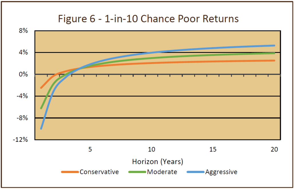
On the other hand, the aggressive portfolio would be expected to have a 1-in-10 chance of generating a return of around -10% in one year. Even the average 2-year and 3-year returns are negative in the worst 10% of cases. The portfolio’s riskiness means that it exhibits very wide dispersion in returns. Even for the highest-return portfolios, there is still a chance of falling short of the 5.25% target over long periods of time. Note that if the expected return on the mix is below the target, the time-period math still works the same. However, in this situation, the likelihood of achieving or exceeding the target declines as the time horizon is extended further in the future (as shown by the orange line in Figure 5).
One of the main implications of this analysis is that riskier/higher return portfolios are appropriate for investors with longer time horizons, despite the greater likelihood of poor returns over shorter time periods.
Conclusion
Many investors hold assets in order to cover future liabilities: individuals for retirement or children’s education; corporations, multi-employer organizations, and governments for pension commitments; foundations for legal spending requirements. Typically, the asset pool needs to achieve a specified rate of return in order to fully fund the liabilities when they come due. By investing in a portfolio with expected returns above the target (required) return, there is a better-than 50-50 chance of achieving the target. In addition, the probability of meeting or exceeding the target improves as the time horizon is lengthened. However, boosting the expected rate of return comes at a cost. Assets with higher expected returns also have higher risk (variability in returns). As a result, there is a possibility that the portfolio will suffer below-target returns (and possibly even losses), even over extended periods of time. This must be considered against the probability, which becomes ever greater over longer periods, of not meeting the return objective with a portfolio that has an expected return that is below the hurdle.
Baseball provides a good analogy to the investment issues discussed above. Think of the conservative low-risk low-return portfolio as akin to a team whose batters swing softly, hoping to just hit singles. Over the course of a full game, getting one or two singles each inning (consistent with assuming the batters’ averages are around 0.250- 0.300) is unlikely to lead to sufficient runs to win the game. If the batters take more “risk” at the plate, swinging harder and trying to hit doubles and triples, batting averages might decline somewhat. But, the chances of getting extra bases increase, as do the odds of getting those runners across the plate and winning the game. As the batters get highly aggressive and “swing for the fences” on every pitch, the likelihood of hitting home runs increases. Unfortunately, the likelihood of striking out rises too. As a result, the “home run” team will play many more games that result in high scores, and many more games that result in very low scores – depending on whether swinging for the fences worked or not.
In building a successful baseball team, it makes the most sense to include a diversified array of batter types – some singles hitters, some who swing for the fences, and others who often hit doubles. In an analogous way, portfolios should be constructed with a diverse array of asset classes – some low-risk bonds, some higher-risk bonds, US equities, developed and emerging non-US equities. This portfolio of assets should, over time, provide investors with a good chance of “winning the game” (i.e. achieving their investment objectives).
Stairway Partners, LLC © 2020
This material is based upon information that we believe to be reliable, but no representation is being made that it is accurate or complete, and it should not be relied upon as such. This material is based upon our assumptions, opinions and estimates as of the date the material was prepared. Changes to assumptions, opinions and estimates are subject to change without notice. Past performance is not indicative of future results, and no representation is being made that any returns indicated will be achieved. This material has been prepared for information purposes and does not constitute investment advice. This material does not take into account particular investment objectives or financial situations. Strategies and financial instruments described in this material may not be suitable for all investors. Readers should not act upon the information without seeking professional advice. This material is not a recommendation or an offer or solicitation for the purchase or sale of any security or other financial instrument.


You must be logged in to post a comment.